eye detector again

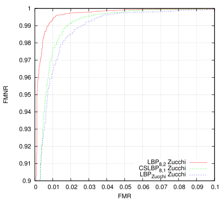
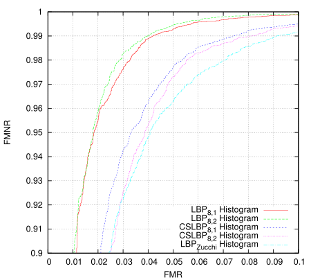
I was playing around with generating ROC curves for various algorithms - first I was trying to determine whether some new LBP codes I came up with worked better in certain cases (not yet, but they have promise, ok i kept playing as below: maybe they do already). For this purpose I implemented a basic LBP histogram matching algorithm, as I figured having baseline would provide a decent comparison.

This just took all eye images as one class and all non-eye images as another and then measured the distance of them all to the classifier. I'm using 20x20 images and the classfier creates 16 histograms from 8x8 tiles overlapping by half in each direction. It isn't terribly valid as a measure because it is using the same set for training and for testing but i'm only after the relative results. There are 10560 positive training examples and 9940 negative examples in the data set, all taken (and synthesised) from Color FERET fa partition. I'm only using abs difference as the distance measure which isn't ideal, and perhaps the 8x8 tile area isn't a large enough sample to build a decent histogram - in short, these histogram results are not tuned for performance.

The Zucchi LBP is using some directional differential filters in order to build the LBP code bit-planes. The idea is that they're tunable to the problem, should be more robust to noise, and generally produce a more noise-free and accurate LBP code. They are much more expensive to calculate however. This tunability offers another possibility for GA optimisation. I guess this is something else I should really write up properly.

Then I revisited the classifier I came up with late 2012 (the one I put into a small android app). Here the data and LBP transform are the same, only the algorithm has changed.

Blew me away a bit, I really didn't expect that much of an improvement. The 'Zucchi' algorithm requires a tiny fraction of the storage and fewer cpu instructions to process. Training takes more memory but fewer instructions per pixel. The original goals in designing it were for it to be SIMD parallelisable (at execution time) so it optimises very well. The first algorithm should be more robust to registration errors, but on this test the differences are remarkable and in many cases you don't want/need such robustness.

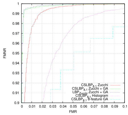
Then I wondered if this classifier could be trained using GA instead. Here I truncated the training set to 8192+8192 images to match the OpenCL GA algorithm, so the results are slightly more valid.

Somewhat surprisingly given the size of the problem (each individual is ~6K bits) it works extremely well and attains a result in only 300 generations. Actually the problem I have is that it is almost too good(tm) - before doing much of a search of the problem space the utility of the fitness measure has been exhausted and the population no longer evolves. One might also note that this result is for the relatively information poor 4-bit LBP codes, and in all cases is only a single-stage classifier.

Given the results I should probably look at the data that isn't classifying properly at each end, some of it may just be poor / incorrectly labelled data. Update: I had a look - the false negatives at the upper end are from synthesised images some of which are over-rotated or rotated off-centre. A couple of the false positives are samples taken a bit too close to the eye although most are legitimate and from around under the nose to under the mouth.

The 8-feature test as described in the previous post doesn't fare so well here - even though it is an effective eye detector in practice and requires about 1/3 of the processing.

Here the differential LBP code is working very well too. And it works extremely well as an eye detector in practice.

For this post I wasn't going to run the differential LBP codes through the GA algorithm based on the first plot - it didn't seem that good. But the final plot and this eye detector heat map somewhat validates the initial reasoning behind the algorithm - reduced noise. See the previous post.

Looking closer at the LBP code image I now see there isn't enough similarity between the left and the right eye regions in the LBP domain to try to create a classifier which resolves both at the same time. What I might do instead is create separate classifiers but not include the other eye in the negative training set - this should improve the results of both. I guess i'm near the point where spectacles should be added to the mix.

I've started writing some of this up but i'm a bit lazy to put the effort in required to do a good job. Apart from the fact that i'm only doing this for self education and entertainment purposes in my spare time right now, i've little experience writing papers. I'm purportedly on holidays for that matter - technically i'm even unemployed but literally i'm just between contracts.

Update: Oops, looks like I made a bit of a mistake. I thought I was using a decent resampler whilst generating the scaled training data, but it wasn't - so aliasing was creating noise in the small-scale images and thus in the LBP codes. This is probably why the derivative LBP code managed to win out in the end. This mistake will lead to the plots showing poorer performance than they should be - but i'm not going to re-run the plots right now.

Seeing that the classifier was doing such a good job, I thought i'd push it a bit harder. I have a couple of other ideas too but the first one I tried was to create a classifier for a very small region. This has very large implications on execution time. So whilst working on an 8x8 classifier I noticed the aliasing and realised the scaling problem. I still have an issue with pixel-boundary sampling when extracting the normalised eye so the data is of a lower quality - but it has to deal with these problems in the input data too.

An 8x8 detector is absurdly small. Here's an example of a decent training image from the training set:

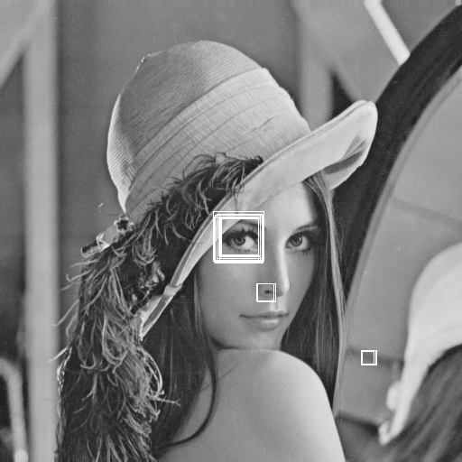
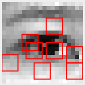
Testing on Lenna's photograph gives quite a few false positives - but out of 181 244 tests, 30 or even 100 false positives isn't too bad for a single-stage classifier. An 8x8 classifier requires 16x less total processing from the inner loop vs a 16x16 classifier to detect the same sized features at the same input scale - so even a modest true negative rate could be a big win if it is reliable. And this doesn't count the image scaling and LBP operator both of which also scale at an N*N rate.

This is just one run of a single-pass 8x8 detector generated via a GA using left and right eye images as the positive set. The threshold was chosen roughly. There are a total of 43 hits out of a total of 181 244 probes, with a false acceptance rate of 0.022%. It took about an hour to generate this detector via pure-Java code on a 6-core intel machine.

This is one run of a single-pass 20x20 detector generated via GA using left-eye images as the positive set. It is being executed over a wide range of scales from 0.2x to 1.5x of the original (512x512) source. There are a total of 22 hits out of a 5 507 592 probes, with a false acceptance rate of 0.00016%. It took about 3 minutes to generate the classifier using the same pure-Java code on the 6-core intel at which point evolution stopped due to having a perfect classifier on the training data set. It took under 200 generations on the improved input data vs the numbers in the top-half of this post.

Update 2: I wasn't going to, but I compared it to the raw results from the left-eye cascade from OpenCV - i remembered it not being particularly good but wanted to quantify it. This is showing the raw hits as exit the cascade and do not include grouping which would remove most of the false positives. There are 313 total hits.

For comparison purposes I re-ran the 20x20 classfier with settings that result in about the same number of scans at roughly the same scales. Here there are 64 total hits, although I just chose an arbitrary threshold value (a fairly loose one however). Haar cascades only provide a binary true/false result and have no threshold that can be adjusted - they also provide no quality indicator so there is no way to choose a peak match and one must resort to error prone averaging and merging.

This code executes about 30% faster than the haar cascade although perhaps the looseness of the haar detector would allow it to be run on fewer locations at the cost of accuracy. However; accuracy is often important if not critical. It should be possible to train a better haar-cascade but I haven't had any luck geting even close to the ones supplied in OpenCV. Likewise this is still only a single-stage classifier and can still be improved (I think) quite easily.

One last data point - the 8x8 classifier over similar scales executes 10-20x faster. These classifiers also scale much much better on parallel hardware - all the way from SIMD to multi-stream GPUs, so this 30% figure is a little misleading. It would also take only a tiny bit of FPGA logic ...

eye detector

I thought i'd see how well the detector works on more general data so first I cleaned up the data a bit and ran against a test image. I cleaned out some closed eyes and excessive squint, mis-alignment, and fiddled a bit with the ratio of eye-size to region. I ended up going with a 20x20 region because adding a bit more height to the classifier seems to help with nose and mouth false-positives. I synthesised a number of rotated images but kept the scale fixed, and included both left and right eyes in the positive training set.

In short, I trained a classifier for open and straight-on eyes only, with a small amount of head tilt (+- 15 degrees) and only misalignment variation to the scale. No spectacles.

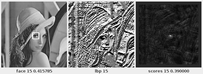
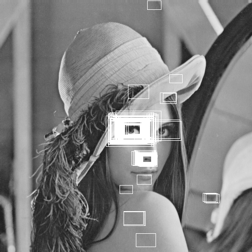
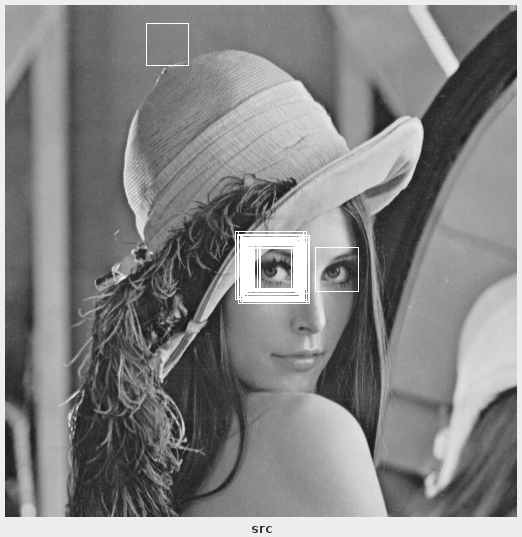
This is the raw results after running the detector over 19 scales from 0.2 to 0.5 of the original Lenna image. The scale range isn't chosen arbitrarily obviously. Whilst the threshold can be adjusted to remove the false positive I left it in to demonstrate some remaining issues. Although blank areas aren't that big of a problem as they can be detected via other means such as variance.

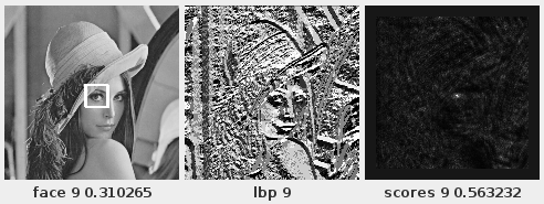
This was the single highest response from all scales tested. The heat map is rendering exp(score), and the result is normalised to highlight the peaks more clearly. The signal being processed is the local binary pattern (LBP) image in the centre, which is a 4-bit CS-LBP 8,1 operator with pixel centered sampling.

As can be seen, It's very good at picking out Lenna's right eye ... her left eye is a bit obscured and off-angle and generally gives the detectors i've tried a bit of grief. It doesn't work well with outside images due to squint, or portraits against a blank background (blank areas score well). But given all of the negative training data come from only face images, it's working quite well as suppressing non-eyes. It has some problems with scale - once the face is about 2x the size the detector expects it starts to pick up eyebrows/noses/mouths/under-eyes but again given the training data this is to be expected - and generally the eye detector is only run after you have face candidates.

This is just with a single 8-feature (4x4) classifier which processes a 20x20 region. I had intended to create a multi-stage classifier but I got side-tracked.

This is the regions used by the classifier created in this example, overlayed with one of the positive training images. The data comes from Color FERET. Any significant overlap is essentially wasted processing (apart from a weighting factor of the overlapped region), so in this case the ga may not have chosen the best solution. It may be worth investigating whether I can get better results by pre-locking the regions and just letting the genetic algorithm choose the other classifier parameters instead.

It took a few runs of the classifier to get a this good result - although the ROC curve fitness measure works well, each run tends to 'lock on' to specific feature points and so that limits the performance to a local peak. If a random bit-flip hits the coordinates it just creates a poorer classifier and it dies immediately.

Some earlier trials had greater problems with background but this particular one was looking very good after about 1K generations so I just kept letting it run for much longer to see if it would get better - it did slightly and the first individual reached 'perfection' on the training set after about 55K generations (around 40 minutes, 8K of each class). Although that wasn't necessarily the best classifier in practice.

Experiments on-going ...

CL+GA ML

Got the OpenCL version of the genetic algorithm based classifier working this morning. Actually I think it already worked, I just had a problem with the way I was testing the output. Because I don't have a better sort just yet I forced the image set to be a power of two. I left the breeding code in Java for now so I don't have to deal with random number generation.

With a population of 512 individuals, 4096 total training images (each 32x16), and using 4x4x4 classifiers it executes a little over 100 generates per second. I was hoping for a bit better but I guess a 30x speedup over single-thread cpu is good enough for now - certainly getting to a solution in 10 minutes is better than 5 hours (just a bit).

The largest single processing element is classifying all the images. However; I am re-executing all classifiers, even those which haven't changed. So I can pretty much double the performance with my current generational settings which keeps half each iteration. The only stage which needs to run over all the whole population is the fitness ranking.

Interestingly on one of the first test runs I managed to create a perfect classifier for the training set after about 40K generations (~8 minutes). Apart from data setup i'm not sure how to tweak this to be more general - as there isn't really 'training' involved, just searching for a good solution to fit the data - i can't really cross-verify with a verify set without it just becoming the training set. A multi-stage classifier could use a verification set for adjusting the thresholds though. The quality of the training set is the most critical factor.

I also tried the three different fitness tests again (approximate area under roc, number of true-positives-before-any-false-positive and number of true-negatives before any true-positivies) and it seems the area under the ROC is by far the best measure. I guess it does work after all, and I think I was just looking at bugs before.

I also upped the mutation rate to 5 bits per off-spring. It gives a bit more 'jiggle' as the improvement rate levels off. It still requires multiple runs because each solution is different, but it seems to help it stave off stagnation for a bit longer. I thought I had a problem with breeding making too many clones of the best solution after a while; but after putting in some checking code I was only ending up with 0-10 clones in any given generation which isn't enough to care about.

I guess I will keep working toward some sort of object detector to see if everything holds up in practice, but i'd like to experiment a bit too - finding time is always the problem.

multi-stage

Cause I was stuck a bit with the OpenCL conversion I tried manually creating a multi-stage classifier to verify it would work.

Given a set of training data I trained a classifier, and then used that to partition the training data - very good true positives or negatives were removed. I then repeated this 3 more times. The final negative data set consists of just 52 images that are very eye-like in the LBP domain: bits of mouth and under the nose. I started with about 4000 negative images and 1000 positive images.

For a fitness score I was maximising the number of false positives with a score better than the worst true positive. This created an ROC curve that rises relatively slowly to start with but keeps rising to a full-pass rate at a fairly low FPR (false positive rate). This isn't normally the ROC curve one seeks because it tends to include plenty of false positives but since i'm seeking to partition the data for a separate stage i'm after the lowest threshold that achieves a TPR of 1 and rejects as much as possible, not the highest TPR vs FPR.

Anyway - it was quite successful, and by 4 stages it had essentially created a perfect classifier to partition that data-set. Each stage tests 4 groups of 4x4 pixels so it only requires a fairly modest amount of work and a very small amount of memory to describe the entire classifier (9*4*4*4 = 576 bytes total). Being a cascade it only processes all stages a small fraction of the time as well.

Of course this is a little too specific to be useful and the training data-sets also need some tweaking - pose and minor scale variation for the positive set and more problematic images for the negative set. So more setup work and experimentation is still required but i'm fairly sure it'll still work on a more general problem.

I got a bit messy with the code and added some big bugs which caused no end of frustration. One I think had been there from the start in certain code-paths - I was showing the LBP image in a window and as part of that it was converting the code to 8 bits not only for display but also for the stored codes. Lets just say this breaks the algorithm although not nearly as much as I would have expected. As part of the OpenCL version I was ordering the scores differently - based on integers and using bitfields to keep track of other info, and I inadvertently added back the bug which interferes with the sort order. Both of these combined to causing the reported success rate to keep climing even though the classifier was just getting worse - what was more confusing is that over time it tended to increase in quality and then start to decline - but only after about 1/2 an hour of processing.

not extending bitonic sort to non-powers of 2

Update: Turns out I was a bit over-optimistic here - this stuff below doesn't work, it just happened to work for a couple of cases with the data I had. Bummer. Maybe it can be made to work but maybe not, but I didn't have much luck so I gave up for now.

Original post ...

This morning I started having a look at combining the OpenCL code I have into a GA solver. Which mostly involved lots of bug fixing in the classifier code and extending it to process all classifiers and images in a single run.

All went fine till I hit the sort routine for the population fitness when I found out that the bitonic sort I wrote doesn't handle totals which are non-powers of two.

e.g. with 11 elements:

input : b a 9 8 7 6 5 4 3 2 1
output: 1 2 3 7 8 9 a b 4 5 6 
        --------------- +++++

Each sub-list is sorted, there is just a problem with the largest-stride merge. I noticed that this merge processes indices:

  0 -> 8
  1 -> 9
  2 -> 10

data  : 1 2 3 7 8 9 a b 4 5 6 
        a a a           b b b

Which misses out on comparing 3-7, which are already going to be greater than 0-2.

So a simple solution is just to offset the first comparison index so that it compares indices 5-7 to indices 8-10 instead. The calculation is simply:

  off = max(0, (1 << (b + 1)) - N); // (here, b=3, N=11, poff = 5)

Which results in the correct merge indices for the largest offset:

data  : 1 2 3 7 8 9 a b 4 5 6 
                  a a a b b b

So an updated version of the sort becomes:

  lid = local work item id;
  array = base address of array;
  for (bit=0; (1<<bit) < N; bit++) {
    for (b=bit; b >= 0; b--) {
      // insertion masks for bits
      int upper = ~0 << (b+1);
      int lower = (1 << b)-1;
      // extract 'flip' indicator - 1 means use opposite sense
      int flip = (lid >> bit) & 1;
      // insert a 0 bit at bit position 'b' into the index
      int p0 = ((lid << 1) & upper) | (lid & lower);
      // insert a 1 bit at the same place
      int p1 = p0 | (1 << b);

      p0 += max(0, (1 << (b+1)) - N);

      swap_if(array, p0, p1, compare(p0, p1) ^ flip);
    }
  }

I haven't extensively tested it but I think it should work. It doesn't!

I'm probably not going to investigate it but I also realised that a serial-cpu version of a bitonic sort wouldn't need to frob around with bit insertions in the inner loop; it could just nest a couple of loops instead. Actually I may well end up investigating it because a similar approach would work on epiphany.

parallel prefix sum 2

This morning I had a quick look at the next stage of the OpenCLification of the GA code. This requires trying to create a fitness measure from the raw score values.

I'm using a sort of approximation of a sum of the area under the ROC curve:

  for each sorted result
    sum += true positive rate so far - false positive rate so far
  sum /= result.length

This gives a value between -0.5 and +0.5, equating to perfectly incorrect ROC and perfectly correct ROC curve respectively. Like the ROC curve itself this calculation is independent of the actual score values and only their order and class is important.

At first I didn't think I would be able to parallise it but on further inspection I realised I could implement it using a parallel prefix sum followed by a parallel sum reduction. The first prefix sum calculates the running totals of the occurance of each class (positive training examples, negative training examples). These values are then used to calculate the two rates above and from those partial summands which are then parallel summed. Because I don't need to keep the intermediate results I process this in batches of work-group sized blocks sequentially across each result array and it is a simple matter to accumulate results across blocks internally.

Then I realised I'd forgotten how to implement a parallel prefix sum properly ... it's been nearly 2 years ... as I found out when using a search engine and finding my own rather useless post on the matter comes up on the first page of results. I had a look at the code generator in socles and distilled it's essence out.

Mostly for my own future reference, the simplest version boils down to this:

  lx = get_local_id(0);
  buffer[lx] = sum;
  barrier(local);
  for (int i=1; i < N; i <&kt; 1) {
     if (lx - i >= 0)
       sum += buffer[lx - i];
     barrier(local);
     buffer[lx] = sum;
     barrier(local);
  }

This of course assumes that the problem is only as wide as the work-group or can be processed in work-group sized chunks; which happens often enough to be useful. There is a very simple trick to remove the internal branch but it's probably not very important on current GPU designs. There are also some fairly simple modifications to widen this to some integer multiple of the work-group size and reduce the processing by the same factor but I don't think I need that optimisation here.

I can also use basic parallel reduction techniques to calculate the lowest-positive-rank and highest-positive-rank values, should I want to experiment with them as fitness values.

This is now most of the work required in evaluating each individual in the population which is the main processor intensitve part of the problem. If I had an APU i'd just drop back to the CPU to do the breeding but since I don't i'll look at doing the breeding on the GPU too, so long as it doesn't get too involved.

parallel batch sorting

Had what was supposed to be a 'quick look' at converting the GA code to OpenCL from the last post. Got stuck at the first hurdle - sorting the classifier scores.

I wasn't going to be suckered into working on a 'good' solution, just one that worked. But the code I had just didn't seem fast enough compared to single-threaded Java Arrays.sort() (only 16x) so I ended up digging deeper.

For starters I was using Batcher's sort, which although it is parallel it turns out it doesn't utilise the stream units very well in all passes and particuarly badly in the naive way I had extended it to sorting larger numbers of items than the number of work items in the work-group. I think I just used Batchers because I got it to work at some point, and IIRC took it from Knuth.

So I looked into bitonic sort - unfortunately the "pseudocode" on the wikipedia page is pretty much useless because it has some recursive python - which is about as useful for demonstrating massive concurrency as a used bit of toilet paper. The pictures helped though.

So I started from first principles and wrote down the comparison pairs as binary and worked out how to reasonably cheaply create compare-and-swap index pairs from sequential work item id's.

For an 8-element sort, the compare-and-swap pairs are:

 pass,step 0,1
  pair  binary   flip comparison
   0-1  000 001  0
   2-3  010 011  1
   4-5  100 101  0
   6-7  110 111  1

 pass 1,2
  pair  binary   flip comparison
   0-2  000 010  0
   1-3  001 011  0
   4-6  100 110  1
   5-7  101 111  1
 (pass 1,1 is same as pass 0,1)

 pass 2,4
  pair  binary   flip comparison
   0-4  000 100  0
   1-5  001 101  0
   2-6  010 110  0
   3-7  011 111  0
 (pass 2,2 is same as pass 1,2)
 (pass 1,1 is same as pass 0,1)

One notices that bit 'pass' is all 0 for one element of comparison, and all 1 for the other one. The other bits simply increment naturally and are just the work item index with a bit inserted. The flip rule is always the first bit after the inserted bit.

In short:

  lid = local work item id;
  array = base address of array;
  for (bit=0; (1<<bit) < N; bit++) {
    for (b=bit; b >= 0; b--) {
      // insertion masks for bits
      int upper = ~0 << (b+1);
      int lower = (1 << b)-1;
      // extract 'flip' indicator - 1 means use opposite sense
      int flip = (lid >> bit) & 1;
      // insert a 0 bit at bit position 'b' into the index
      int p0 = ((lid << 1) & upper) | (lid & lower);
      // insert a 1 bit at the same place
      int p1 = p0 | (1 << b);

      swap_if(array, p0, p1, compare(p0, p1) ^ flip);
    }
  }

The nice thing about this is that all accesses are sequential within the given block, and the sort sizes decrement within each sub-group. Which leads to the next little optimisation ...

Basically once the block size (1<<b) is the same size as the local work group instead of going wide the work topology changes to running in blocks of work-size across. This allows one to finish all the lower stages entirerly via LDS memory. Although this approach is also much more 'cache friendly' than full passes at each offset, LDS just has a much higher bandwidth than cache. Each block is acessed through the LDS via a workgroup-wide coalesced read/write and an added bonus is that for the larger sized blocks all memory accesses are fully sequential across the whole work-group - i.e. are also fully coalesced. It might even be a reasonable merge sort algorithm for a serial processor: although I think the address arithmetic will be too expensive in that case unless the given cpu has an insert-bit instruction that makes room at the same time.

On closer inspection there may be another minor optimisation for the first LDS based stage - it could perform the previous stage in two parts whilst still retaining full-width reads using a register.

I'm testing by sorting 200 arrays, each with 8192 integers (which is what i need for the task at hand). I'm using a single workgroup per array. Radeon HD 7970 original version.

  algorithm         time

  batchers          8.1ms
  bitonic           7.6ms
  bitonic + lds     2.7ms

  java sort        80.0ms  (1 thread, initialised with random values)

Nice!

I think? Sorting isn't something i've looked into very deeply on a GPU so the numbers might be completely mediocre. In any event it's interesting that the bitonic sort didn't really make much difference until I utilised the LDS because although it requires fewer comparisions it still needs the same number of passes over the data. Apart from that I couldn't see a way to utilise LDS effectively with the Batchers' sort algorithm I was using whereas with bitonic it just falls out automagically.

Got a roast lamb in the oven and cracked a bottle of red, so i'm off outside to enjoy the perfect xmas weather - it's sunny, 30-something, with a very light breeze. I had enough of family this year so i'm going it alone - i'll catch up with friends another day and family in a couple of weeks.

Merry X-mas!

Update: See also a follow-up where I explore extension to non-powers of two elements.

genetic algorithm experiments

Last couple of days I was playing with some genetic algorithm code to implement an object detector. This is the first time i've ever played with genetic algorithms so is simply exploration to become aquainted with the technique.

First I started with a local binary pattern histogram feature test based on the paper Genetic Based LBP Feature Extraction and Selection for Facial Recognition, but these were just too slow to evaluate to work out whether I was making any progress or not. It wasn't quite the problem I wanted to solve but I did have the paper and am familiar with the algorithm itself.

So I changed to using a variation of my own 'single-bit-histogram' algorithm which is much faster to evaluate both because the mechanics of it's implementation and the mathematics of the fitness determination. Because it generates a classifier and not a distance measure evaluation of fitness is O(N) rather than O(N^2). Initially my results seemed too good - and they were, a simple sort-order problem meant that a completely zero detector came out as perfect. After fixing that I did still have some promising results but my feature tests were just too small so the discriminative ability wasn't very high.

When I left that for the day I didn't think it was really working that well because the feature tests weren't descriptive enough on their own - only a few single probes. But I was looking at the output a bit wrong - it doesn't need to be 'good', it just needs to have a low false-negative rate. The next morning I tried creating a more complex descriptor based on a 4x4 feature test - and this worked much better.

The GA

After reading a few light tutorials on the subject I basically came up with my own sexual and asexual (i.e. copy with mutate) breeding rules and mucked about with the heurstics a bit. Throwing out years of research no doubt but without some understanding of how it works I wont understand it properly. So they are probably not ideal but they seem to work here.

The basic asexual breeding rule is:

1. Randomly grow or shrink the number of genes by 1 (within a specific range);
2. Copy genes, potentially mutating each bit separately;
3. If the chromosome grew, add a new random gene.

And sexual breeding:

1. Concatenate all genes of both parents;
2. Randomly permute the whole set;
3. Choose a new size which is half the combined gene length +/- 1 (within a specific range);
4. Truncate to the new size;
5. Randomly mutate every bit.

Genes are treated 'whole', and it obviously supports different numbers of genes for each individual chromsome. I found that a small number of tests seems to work better than a larger number; at least for the single-pixel classifier. As such i'm focusing at present on fixing the gene count in advance and running multiple tests to see what difference the gene count makes.

I tried a few different fitness tests:

• Order by area under ROC curve (or for simplicity, some approximation thereof);
• Order by rank of first incorrect result;
• Order by rank of last correct result.

These all result in slightly different classifiers - although the first tends to be the best. Combining a couple by simple concatenation also appears to create a better classifier.

Each generation i discard the worst-N results, and then randomly sexually or asexually reproduce random pairs or individuals to replace them. For simplicity i'm just using uniform randomness rather than basing reproduction rates on fitness. I presume at worst this just reduces the rate of advancement.

I need to read up a bit more on the nomclature and jargon used to describe the behaviour properly but with very small number of genes I tend to end up with poor genetic diversity at least in the top few results (I'm dumping the top 5 every 100 generations). I think my random mutation isn't random enough during breeding - it should always mutate at least some bits rather than applying a low randomisation rate across all of them.

Still, even with these shortcomings and the fact that after a rapid improvement progress slows - it doesn't stall completely. I ran some very long experiments and even after 10 hours I was still getting an occasional improvement.

The Classifier

I need to write up the classifier a bit better than a blog post so I wont go into the detail here. I think it's a novel use of local binary patterns.

But the current 4x4 'gene' consists of:

struct gene4x4 {
  unsigned int x:5;
  unsigned int y:5;
  unsigned int pad:22;
  unsigned int tests[8];
};

(x,y) is the location of the test, and the 16x16-bit integers stored in the tests array are the parameters. For the descriptive power it seems to have, this quite a compact descriptor. With a chromosome of as little as 2 of these genes i'm starting to get some interesting results, and at 4 genes I think i'm starting to get usable results. That's only 1024 bits; this is something that can easily fit on an epiphany core even with a good few stages.

Data

As with any machine learning algorithm dataset size and quality is another issue, but for now i'm just using what I have which is stuff i've extracted from Color FERET. The training set is the left (from front, i.e. right) eye at 32x16, and the negative training set is random samples from the same faces excluding those very close to the eye. I'm just using the same set to test against at the moment.

I think though that because of the similarity of the eyes and the fact that you can easily tell them apart using simple geometry I will look at combining left and right eye detectors into a simple 'eye detector'. This saves the learning algorithm the hassles of trying to distinguish between left and right eyes as well as non-eye data. If I really needed to distinguish between the two I could train another detector for sub-classification - to be honest, I can't really see why you would need to.

Next

One thing I want to do is translate the algorithm to OpenCL so I can accelerate the generation rate. I already have the classifier written and that can score images insanely fast - so fast that I think I need to write the whole algorithm in OpenCL now, which wasn't my original intention. Being able to run a few hours worth of testing in minutes really accelerates experimentation with the heurstics and other gene variations so it's worth the day or so of effort it needs to get working.

Then I want to investigate whether I can turn these classifiers into a reliable cascade of classifiers - which is a critical step for both runtime and quality performance. My first thoughts are to use the ROC curve to choose a threshold such that some of the false positives are culled (but no false negatives), remove those from the data-set and then train a new classifier; and repeat until one reaches a satisfactory result. A variation may be to also cull at the true-positive end of the classifier if there is a particularly high first-false-positive rank. My gut feeling so far is that because each classifier is not too weak it shouldn't need too many stages to be very strong; but whether this pans out in practice or not is another matter.

Then there are many things to try, from data improvements / different objects, to adding extra dimensions to the input data (e.g. multiple planes different lbp codes which test for different characterestics; somewhat analogous to multiple gabor wavelets). It should also be possible to directly create a multi-stage algorithm soley using GA - which may be worth investigating.

The ultimate aim is a strong classifier which is also computationally efficient (ahem, yeah, kinda holy grail territory here, i'm not ambitious at all). I know already that it can be implemented in ARM NEON assembly language very efficiently - under 1 clock cycle per pixel tested(!). It's also simple enough to put in hardware. I'm just not sure yet whether I can make it strong enough to compare to other algorithms, which is of course the big question.

On a side note it's kind of cool having the computer just work away by itself coming up with a solution given very simple goals. For once. It normally feels like it's the one driving me.

Of course, being xmas, and being on leave, ... I may just drink wine instead! And it's about time i put down another homebrew. And cleaned the house a bit. Time for another #3 all over too.